My overview of LRM

Introduction

I’ve been updating myself on the most major advancements in the field of 3D reconstruction and text-to-3D over the past year, and I’ve seen lots of tricks to improve performance, reformulate the task in various ways, inserting components from different fields of Machine Learning, and so on.

Recently I saw a paper that described a method called Large Reconstruction Model (LRM) that generates a 3D object from a single image. It just blew my mind with how things like this are possible now. Largely because of the enormous 3D datasets available – Objaverse and MVImgNet

Initially I thought I’d just make a streamlined post with my thoughts on the topic.
Then I thought I wanted to make one large post describing many concepts in 3D generative models – but decided that’s too much for one post, and I’ll burn out before writing something actually good. So I’ll focus on overviewing just this paper I found fascinating.

Overview

So the idea of LRM is a lot simpler compared to those of MVDream / DreamCraft3D / etc. which utilize Score Distillation Sampling (from the DreamFusion paper).

In this paper we’re simply training a model that, given a single input image, predicts a NeRF of the 3D object. That’s it. That’s the idea. The rest is architectural / implementation details. I’ll explain why this is amazing later.

Let’s pull up the image describing their model architecture:

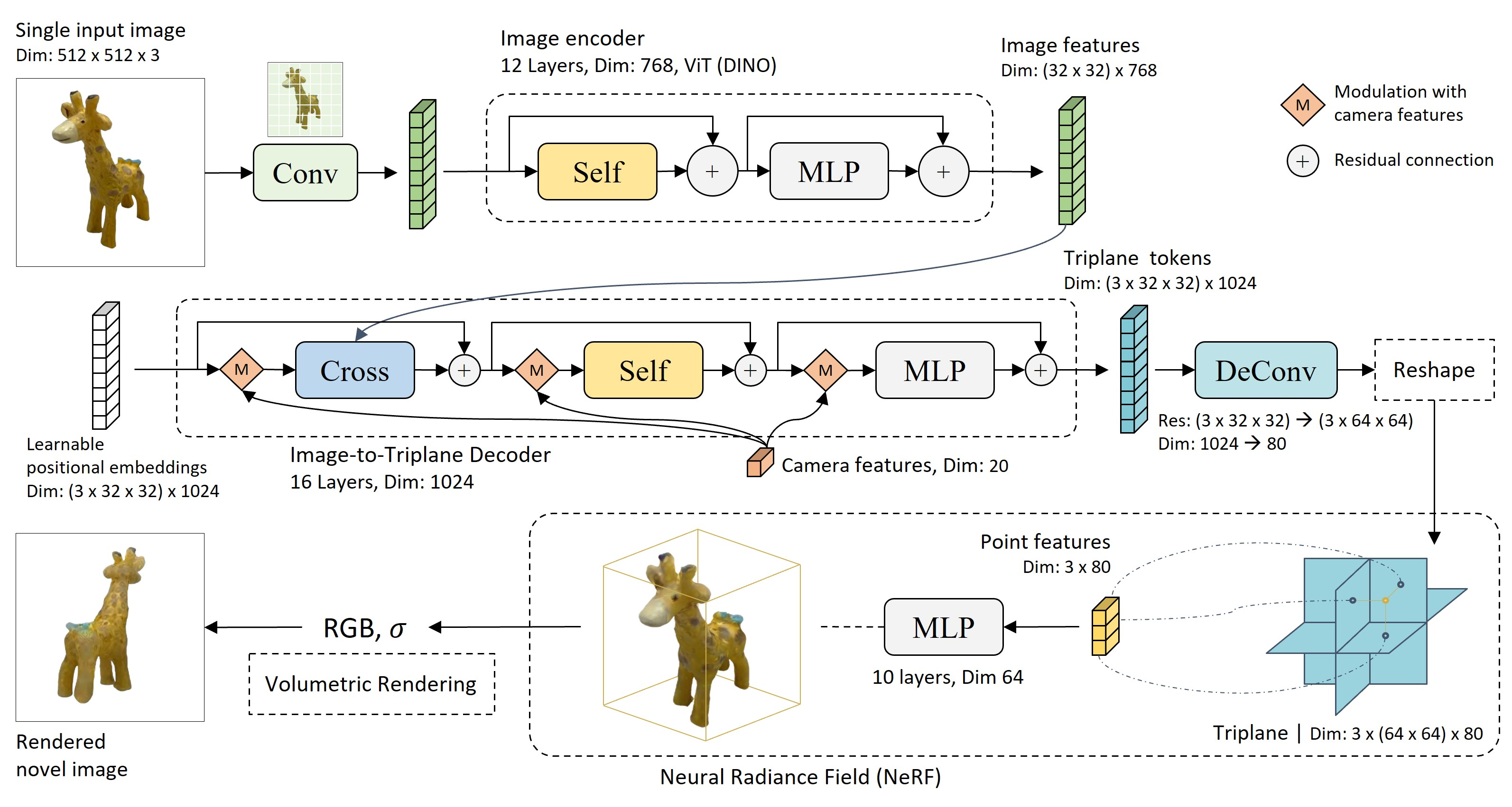LRM architecture from the paper

This is just for reference – it’s some kind of neural network that just does “Image -> NeRF”. How a NeRF can be regressed with a model I’ll explain here.

Let’s start with how whatever this is is trained.

How LRM is trained

All variable names are improvised by me, don’t try to look for corresponding formulas/variables in the paper

\[\begin{aligned} I & \ -\ \ \text{Input image}\\ G_{\phi } & \ -\ \ \text{Large Reconstruction Model}\\ G_{\phi }( I) \ =\hat{\Theta } \ & \ -\ \ \text{The 3D object generated by LRM} \end{aligned}\]

Here I’m denoting the 3D object with $\hat\Theta$, what this is in particular I describe in the 3D representation section.

The way to train this model is pretty trivial if we have the required data: we are trying to solve the image-to-3D issue, i.e. we want to know the mapping from 2D to 3D. BUT – for any 3D object we know the true mapping from 3D to 2D (given camera parameters) – it’s the render of the object.

\[\begin{aligned} c & \ -\ \ \text{Camera parameters}\\ p(\hat{\Theta } ,\ c) \ =\ \hat{I} & \ -\ \ \text{Render of the 3D object} \end{aligned}\]

So let’s just get a dataset of 3D objects, get 2D renders of them, and train the model to do the opposite!

\[\begin{aligned} D\ =\ \{\Theta _{1} ,\ \dotsc ,\ \Theta _{N}\} & \ -\ \ \text{Dataset of 3D objects}\\ \Theta _{i} \in D & \ -\ \ \text{A sample 3D object from the dataset}\\ c & \ -\ \ \text{Random sampled camera parameter} \ \\ I=p( \Theta _{i} ,\ c) & \ -\ \ \text{Render of the sampled 3D object} \ \\ G_{\phi }( I) \ =\ \widehat{\Theta _{i}} & \ -\ \ \text{LRM's estimation of the 3D object} \end{aligned}\]

Though we didn’t specify one thing yet – how are we going to compare $\Theta_i$ and $\hat \Theta_i$? These two (as we’ll see later) are 3D objects that are really hard to compare directly.

Then how about indirectly – via their renders? If two objects looks the same from all sides, you can pretty much consider them identical. So let’s compare the renders of $\Theta_i$ and $\hat \Theta_i$. Though we’ll have to use more camera parameters:

\[\begin{aligned} c_{1} ,\ c_{2} & \ -\ \ \text{Random sampled camera parameters} \ \\ I_{1} =p( \Theta _{i} ,\ c_{1}) ;\ I_{2} =p( \Theta _{i} ,\ c_{2}) & \ -\ \ \text{Renders of the sampled 3D object} \ \\ G_{\phi }( I_{1}) \ =\ \widehat{\Theta _{i}} & \ -\ \ \text{LRM's estimation of the 3D object}\\ p\left(\widehat{\Theta _{i}} ,\ c_{2}\right) \ =\ \widehat{I_{2}} & \ -\ \ \text{Render of LRM's estimation}\\ \mathcal{L}\left( I_{2} ,\ \widehat{I_{2}}\right) & \ -\ \ \text{Loss function for LRM} \end{aligned}\]

Even though $\mathcal{L}\left( I_{2} ,\ \widehat{I_{2}}\right)$ is just comparing two images, sampling many more renders and minimizing this loss for many-many sampled $\Theta_i$ will result in our model producing faithful 3D reconstructions.

As always, the tougher the ML task is, the more & higher-quality data we need. LRM in particular trains on huge Objaverse and MVImgNet that appeared relatively recently, so it’s no wonder it got to this level of quality and consistency.

---

Ok, we have the understanding of what this model is trained to do.
This was the most fascinating part of this method to me – it’s just so straightforward, compared to Score Distillation Sampling methods that rely on a pretrained diffusion model, do various tricks with it, etc.

Now model architecture itself – it has crucial ideas too.
Lots of scary blocks, so let’s go component by component.

NeRF for 3D representation

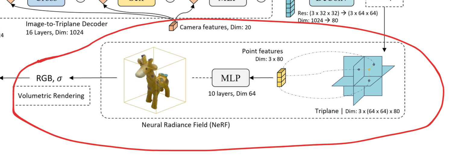A NeRF is predicted via regressing triplanes

Just like most of the current state-of-the-art Image-to-3D/Text-to-3D approaches, this paper generates an object represented as a NeRF. It does so by regressing the planes for the Triplane Encoder that is introduced in TensoRF.

This idea of regressing a NeRF from an input isn’t new – it’s very often used in 3D GANs, where we’d like to generate a 3D object from a latent code. EpiGRAF is a good example – it uses a backbone very similar to StyleGAN2 to generate the 3 embedding images that are reshaped into this Triplane structure.

The MLP is the same for every object – only the Triplane features change, therefore they are the ones driving the geometry & appearance, and the MLP is trained to interpret all those features.

Image Encoder

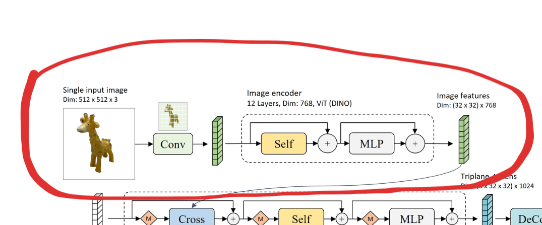Image encoder architecture

Almost always when processing a single image with some type of Neural Network, we want to extract meaningful features for future processing. This paper goes the Transfer Learning path and just uses the image encoder from DiNO (very powerful image embedder trained with self-supervision). Not much else to describe here.

Injecting image features into the Triplane

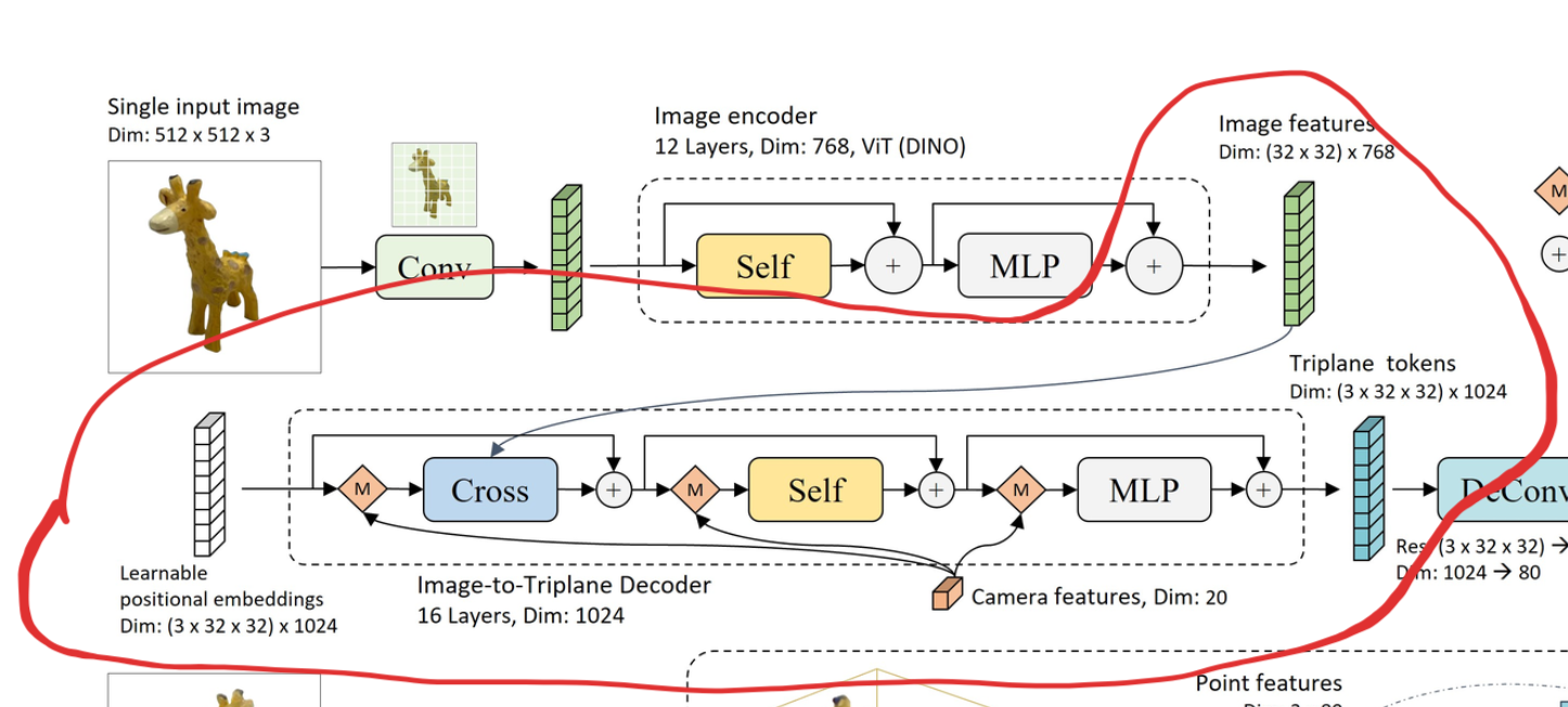Cross-Attention to integrate image features into the triplane

So, on the left here you can see Learnable positional encodings with the shape $(3 \times 32 \times 32) \times 1024$ – you can maybe guess that these positional embeddings are also a TensoRF Triplane, i.e. the 3 images comprising such a Triplane. I called this section “Injecting image features into the Triplane” because we aren’t really predicting those Triplane images – we’re modifying existing ones via Cross-Attention.

The encoded camera parameters are also injected in this decoder, though I don’t find it interesting explaining how exactly they are injected. They just are – to inform the Cross-Attention layers of the n’Point of View of the input image.

Looking at how this transformer with Cross-Attention is implemented isn’t really that informative:

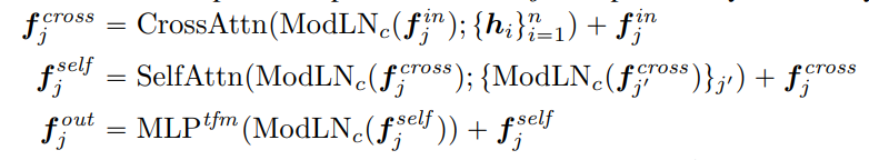The formulas for a single Image-to-Triplane layer

BUUT knowing that there’s 16 layers of this Cross/Self-Attention does make an impression that we’re meta-learning Score Distillation Sampling, i.e. the Attention layers simulate the distillation of image features into 3D.

This is the paper I was thinking about: https://arxiv.org/abs/2212.07677
Basically authors show that Transformers out of Self-Attention blocks resemble “mesa-optimizers”, i.e. modify the input features at every layer to minimize some objective. Didn’t read it through though, just saw a summary of this somewhere 🤪

Noteworthy Technical details

• Ground-truth camera parameters $\mathbf{c}$ are only injected into the Image-to-Triplane decoder during training. During inference, the camera features are replaced with an encoding of the default, fixed camera parameters
• The loss $\mathcal{L}(I, \hat I)$ not only has an $L2$ loss inside, but also an $LPIPS$ loss, often referred to as a Perceptual loss. Empirically, minimization of just the $L2$ leads to blurriness, but $LPIPS$ loss compares features related to local structures, therefore minimizing it leads to better preservation of edges. And an ablation study shows that removing it results in a drop of all metrics.
• Instead of sampling ground-truth renders of data during training, authors sample 32 renders of each object as a pre-processing stage, and then train with those renders only, for optimization purposes
• My favorite – it takes a looooot of hardware to train such a large model on so much data. For them it took 128 A100s training for 3 days, on a batch size of 1024. Nowadays this may seem like a normal workload for a Computer Vision lab, but it’s still mind-boggling to me
• They use deferred back-propagation from ARF , which I learned about just while writing this post. Definitely recommend reading Section 4.2 from their paper that explains how they optimize NeRF back-propagation

To save computational cost in training, we resize the reference novel views from 512x512 to a randomly chosen resolution between 128x128 and 384x384 and only ask the model to reconstruct a randomly selected 128x128 region. With this design, we can possibly increase the effective resolution of the model.

• Basically, the $\mathcal{L}(I, \hat I)$ is actually computed on patches
• An ablation study shows that training without the real images from MVImgNet rapidly drops all of the metrics. Presumably because they have a lot more lighting/size/camera pose variation (though if they sample cameras themselves for Objaverse, why do they say they don’t have enough variation?)

Conclusion

Again, I love how straightforward this approach is compared to the usual Score Distillation Sampling way. And how so much is possible if you have enough GPUs.

Please, if you have any feedback on the post, I’d love to hear it! The comments under the post should work, or you can DM me on Twitter / Telegram.