The CamP NeRF paper is amazing

Sometimes I read papers about NeRF. Yeah, what a shock.

Whatever — point is, most of the time they contain some nice hacks to improve the quality of reconstructions / speed up training / use them creatively for a new kind of task.

For the first time in a reeeeally long time, I’m actually very-very impressed by the ideas presented in a paper about NeRFs. First — because I actually tackled the problem this paper is about, second — this idea is generally applicable to basically any ML scenario.

Also, an important note — I recommend reading all of this only if you’ve read through the paper. Maybe you didn’t understand the idea, or maybe you did — I still think putting all of the intuition into words is very useful for the brain.

CamP: Camera Preconditioning for Neural Radiance Fields
https://camp-nerf.github.io/

Introductory thoughts

Basic ideas as preliminaries to the main idea:

• Usually camera positions for NeRF are obtained with COLMAP, pretty old-style Computer Vision software for estimating scene geometry and camera parameters from a large set of photos 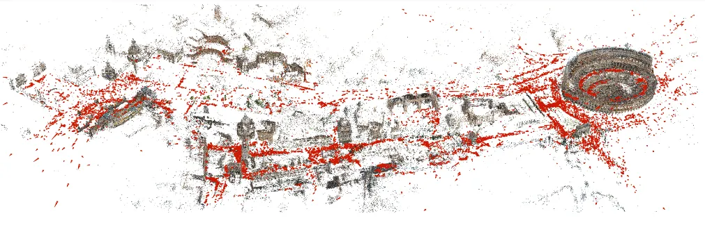COLMAP: Reconstruction of the area around the Colloseum from lots of tourist photos

• Sometimes these estimated cameras aren’t perfect — they may be an infinitesimall unit away from the true camera parameters
• Some NeRF methods already implement fine-tuning camera parameters during the reconstruction process. Bundle-Adjusting NeRF was the first one to do so, NeRFStudio’s default method nerfacto implements pose refinement.
• But both methods from above only refine camera poses, i.e. their translation and rotation parameters. But those are relatively easy to optimize with Gradient Descent, compared to, say, the Focal Length of the camera

Intuitively, the Focal Length behaves badly because of how it affects projected poins:

Different frameworks define the intrinsic matrix differently, but this is usually how formulas for projection of a point to a camera look:

\[\begin{aligned} p_{\text{world}}\in\mathbb{R}^3 \quad &- \quad \text{point visible by the camera}\\ R\in\mathbb{R}^{3\times 3}, T\in\mathbb{R}^{3} \quad &- \quad \text{extrinsic rotation and translation of the camera}\\ f\in\mathbb{R}_+\quad &- \quad \text{focal length}\\ K = \begin{pmatrix} f & 0 & \frac{1}{2}\\ 0 & f & \frac{1}{2}\\ 0 & 0 & 1 \end{pmatrix} \quad &- \quad \text{the intrinsic matrix}\\ p_{\text{camera}} = Rp_{\text{world}} + T = \ \begin{pmatrix} x\\ y\\ z \end{pmatrix} \quad &- \quad \text{point transformed to camera space}\\ p_{\text{screen}} = Kp_{\text{camera}} = \begin{pmatrix} xf\ +\ \frac{z}{2}\\ yf\ +\ \frac{z}{2}\\ z \end{pmatrix} \ \quad &- \quad \text{homogeneous projection} \end{aligned}\]

“homogeneous“ here means that the 3rd component is the depth. And dividing the whole vector by that depth is basically the operation that gives the perspective effect — coordinates of objects with larger depths will be divided by a larger value, therefore the object will become smaller:

I reeeally enjoyed making all these LaTeX formulas, but I got a little off-topic. 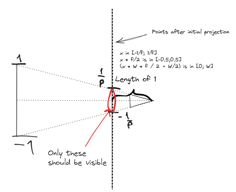An old drawing of mine I made to derive the values in the intrinsic matrix

The point is (or, my intuition is) — the translation & rotation matrices affect the projections of points in a pretty straightforward manner. Move the camera’s position with some vector — the projections will move by something proportional in magnitude to that vector (if we assume that the parallax effect isn’t too strong). The rotation similarly affects points by some vector with magnitude proportional to a sine/cosine or whatever of the angle change.

Whereas the focal length stretches points very non-uniformly over the image space. And changes to the focal length when it’s 2 or when it’s 10 will have a different absolute effect on the projection coordinates. Which means that it affects the projections very differently compared to the translation / rotation.

And this difference is what hinders simultaneous optimization of all camera parameters — at least, my lots and lots of experiments showed so. The focal length either optimizes too slowly or diverges, because there is no single good learning rate for it, when at every point in optimization it kind of needs a new one.

Aaaaand this leads us to what the paper actually does

CamP NeRF — how to optimize all camera parameters at once

Let’s get right to the idea I’m fascinated about.

In the previous section, what did we use to explain how the focal length affects different points differently? Riight — the different points.

So let’s just look at the gradient of the camera parameters with respect to some points sampled in our volume:

\[\begin{aligned} p\in \mathbb{R}^{3N} & \quad -\quad \ \text{sampled points}\\ \phi \in \mathbb{R}^{M} & \quad -\quad \ \text{camera parameters}\\ \Pi ( \phi ) =p_{\text{proj}} \in \mathbb{R}^{2N} & \quad -\quad \ \text{projection function}\\ \frac{\partial \Pi }{\partial \phi } =J_{\Pi } \in \mathbb{R}^{2N\times M} & \quad -\quad \ \text{Jacobian of the projection function} \end{aligned}\]

Ok so this should be relatively understandable — this Jacobian literally contains the effect of each camera parameter on each of the points’ coordinates.

Now, let’s fantasize a bit — what properties of this Jacobian would make this perfect for Gradient Descent? First off — we already talked about how difficult it is to pick the right learning rate, when all parameters affect the inputs with different scales. So:

1. Force the magnitude of each column of this Jacobian to be some constant

Another nice property you could think of if you had 200 IQ or if you had foresight — it would be so great if the effect of our camera parameters was decoupled. By that in Linear Algebra it usually means that we want some vectors describing change to be orthogonal. So basically

1. Force different columns of this Jacobian to be orthogonal

Both of these properties on the columns of the Jacobian can be conveniently explained over this matrix:

\[\begin{aligned} \Sigma _{\Pi } \ =\ J_{\Pi }^{T} J_{\Pi } & \quad -\quad \ \text{matrix of dot products of the Jacobian columns}\\ ( \Sigma _{\Pi })_{ii} & \quad -\quad \ \text{magnitude of the } i\text{-th column}\\ ( \Sigma _{\Pi })_{ij} & \quad -\quad \ \text{dot product of columns} \ i,j \end{aligned}\]

It’s simple but it works — to satisfy our properties 1 and 2, we would just need this matrix to be uhhhh I don’t know THE IDENTITY MATRIX.

Now, if you’ve read through the paper, you understand that it’s all about modifying the camera parameters in such a way that they would behave better for Gradient Descent. Up above, we just explained what needs to happen for the camera parameters to behave well.

And the authors make it pretty easy — they just multiply the camera parameters by a matrix and show how all of the above properties are suddenly satisfied. It’s fun to lay all of this out on paper, so if you have time and brain power to do this, I definitely encourage you to.

Best thing about this whole discussion in this section — never once did we even use the fact that this is a camera. Points can be something different, the camera can be a completely different set of parameters. This idea of equalizing the gradient magnitudes for all of the parameters is applicable ANYWHERE. Jk — only in places where this Jacobian is relatively easy to compute, and there’s only a few parameters, so the matrix inversion that is used in one of the formulas is cheap.

Concluding words

This wasn’t a very exhausing explanation of the paper. It was more like a concentrated flood of my excitement about an idea from the paper. And I really like being very excited about stuff and trying to explain it!

I always appreciate feedback

Peace!